Research funded by EU Framework Program 7

22 Nov 2016
By Märt Toots
visualization

In this post we are mapping the collaboration networks between European research institutes, based on the European Union Framework Program No.7 (2007-2013) funded research projects data. The post is a bit lengthy but the outcome looks good in my opinion.The datasets are taken from the European Union open data portal featuring thousands of freely available datasets. I chose the framework program 7 (FP7) dataset just because it was the latest complete dataset. The next funding program Horizon 2020 lasts until, well 2020, and includes thus less datar.

Let’s get going

# Load libraries

Let’s strat by loading some libraries

# Useful piping operators
library(magrittr) 

# Data manipulation and ggplot2
library(tidyverse)

# String manipulation
library(stringr)

# Plotting maps
library(maps)

# Computing geodesics
library(geosphere)

# Handling dates and times
library(lubridate)

# For handling requests to Google Maps API
library(RCurl) 
library(RJSONIO)

Data import

I have a couple of interesting datasets.

countries - Table between ISO country codes and long country names
fp7org - The main dataset. It includes all of the institutions that were participants in any of the research projects funded from fp7 funds. It also includes the addresses and how the contribution from fp7 were divided between the institutions.

Countries

Start by importing countries. The data can be scraped from a html table here using R library rvest

library("rvest")

page <- read_html("https://developers.google.com/public-data/docs/canonical/countries_csv")
countries <- page %>%
  html_nodes("table") %>% 
  .[1] %>% 
  html_table() %>% 
  .[[1]] %>%
  as_data_frame() %>%
  select(-latitude, -longitude)

#Fix Namibia, whose code NA is treated as missing value
countries[countries$name == "Namibia", "country"] <- "NA"

It turns out that the country codes in fp7 dataset are European codes, so let’s some of them to ISO in order to join with the countries dataset

countries <- countries %>% 
  #Change ISO code to EU code --->
  mutate(country = str_replace(country, "GB", "UK")) %>%  #UK
  mutate(country = str_replace(country, "GR", "EL")) %>% #Greece
  mutate(country = str_replace(country, "XK", "KO")) %>% #Kosovo
  mutate(country = str_replace(country, "RS", "CS")) #Serbia

FP7

Next, let’s import the main dataset. A couple of notes

The dataset includes institution names in a variety of different languages so we have to make sure we get the data as UTF-8. I had to jump through some hoops to get everything correct
In Europe it is common to write , as a decimal separator, so this has to be specifies
project with a reference number rcn == 88383 had several times larger contribution that anything else, so I’m omitting it. I think it’s some kind of a separate grant fund or something

fp7org <- read_tsv("../assets/posts_data/2016-11-22/fp7org_utf8_tsv.txt", 
                   locale = locale(decimal_mark = ",")) %>%
  
  #Throw out unneeded variables and rename some others
  select(rcn = projectRcn, 
         ref = projectReference, 
         acronym = projectAcronym,
         role, name, country, street, city, postCode,
         contact_title = contactTitle,
         first_name = contactFirstNames, 
         last_name = contactLastNames, 
         activity_type = activityType, 
         contr = ecContribution) %>%
  
  #exclude an outlier
  filter(!rcn %in% c(88383))

Data cleaning

Turns out there are some duplicate entries in the dataset. Let’s remove them

#remove duplicates
fp7org <- fp7org[!duplicated(fp7org), ]

Join fp7org with countries to get the country names

#Add country names
fp7org <- fp7org %>%
  left_join(countries, by = "country") %>%
  select(name = name.x, country_name = name.y, everything())

I am interested in the city level address of each of the institutions. But it is a rather messy dataset. Need to fix some obvious things

#Fix city names
fp7org <- fp7org %>%
  mutate(city = tolower(city)) %>% #All to lower case
  mutate(city = str_replace_all(city, "[\"\'\\?\\.]", "")) %>% #remove some punctuation
  mutate(city = str_replace_all(city, "[0-9]", "")) %>% #replace numbers with empty string
  mutate(city = str_replace_all(city, "#name", "")) %>% #Some have this as a name
  mutate(city = str_trim(city))#Trim white from both ends

#Combine city and country to address. Do some cleaning
fp7org <- fp7org %>%
  mutate(city_adr = str_c(city, country_name, sep=", ")) %>%
  #if there is no city specified, then use only country name
  mutate(city_adr = ifelse(is.na(city) | city == "", country_name, city_adr))

Get city coordinates

Query the city coordinates from google maps API. I could use a join with the world.cities dataset provided by the maps package, but the city names are really messy and relying on googles fuzzy matching is much more reliable.

To connect to Google Maps API I adapted the code from here to my liking.

Converting and address into the longitude and lattitude coordinates is called geocoding. The number of free request per day is 2500 at a rate of 50 requests per second. If one of those limits is exceeded the service responds with OVER_QUERY_LIMIT. To avoid that I did 2500 requests per day and waited 1/5 of a second between each request. It’s an overkill but waiting shorter time sometimes still ended in exceeding the query rate. Anyway, we have here around 10000 city addresses so the whole process took 4 days.

cities <- fp7org %>%
  filter(!is.na(city_adr)) %>%
  count(city_adr) %>%
  mutate(lat = NA, lon = NA, 
         location_type = NA, 
         fixed_adr = NA, 
         status = NA)

#Google API allows 50 requests per second.
#Stay on the safe side and sleep 1/5th of a second
between_requests <- duration(1/5, "seconds")

#Function to construct the request to the API.
# NOTE: use your own apiKEY
url <- function(address, return.call = "json") {
  apiKEY <- "xxx-xxx-xxx-xxx"
  root <- "http://maps.google.com/maps/api/geocode/"
  u <- paste(root, return.call, "?address=", address, "&apiKEY=", apiKEY, sep = "")
  return(URLencode(u))
}


# Query the next bunch of addresses until OVER_QUERY_LIMIT
#Daily limit 2500
for(i in 1:nrow(cities)){
  
  #Only for those that have not been queried yet
  if(is.na(cities$lon[i])){
    print(paste0("checking ", i, ": ", cities$city_adr[i]))
    
    #get the request url
    u <- url(cities$city_adr[i])
  
    #Wait in order to stay below query rate limit
    Sys.sleep(between_requests)
    
    #Send the request/get the response
    doc <- getURL(u)
    
    x <- fromJSON(doc, simplify = FALSE)    
    
    if(x$status == "OK") {
      print("> status OK")
      
      #Parse the results
      lat <- x$results[[1]]$geometry$location$lat
      lon <- x$results[[1]]$geometry$location$lng
      location_type <- x$results[[1]]$geometry$location_type
      formatted_address <- x$results[[1]]$formatted_address
      row_result <- c(lat, lon, location_type, formatted_address, "OK")
      
      #Add to the dataframe
      cities[i, 3:7] <- row_result
      
    } else if(x$status == "OVER_QUERY_LIMIT") {
      print("> over query limit")
      break
      
    } else {
      print(paste0("> status: ", x$status))
      cities[i, 3:7] <- c(NA, NA, NA, NA, x$status)
    }
  }
} 

#When finished, save the RDS
#saveRDS(cities, file = "dat/eu/cities.rds")

Exploration

Glimpse the cities dataset

cities %>% glimpse

## Observations: 9,587
## Variables: 7
## $ city_adr  <chr> "a coruna, Spain", "a coruña, Spain", "aabyhoej...
## $ n         <int> 15, 1, 1, 1, 407, 2, 4, 1, 181, 3, 1, 1, 3, 2, ...
## $ lat       <chr> "43.3623436", "43.3623436", "56.1565195", "56.1...
## $ lon       <chr> "-8.4115401", "-8.4115401", "10.1689744", "10.1...
## $ precision <chr> "APPROXIMATE", "APPROXIMATE", "APPROXIMATE", "A...
## $ fixed_adr <chr> "A Coruña, Spain", "A Coruña, Spain", "Aabyhoj,...
## $ status    <chr> "OK", "OK", "OK", "OK", "OK", "OK", "OK", "OK",...

As we can see, there are at least two ways how A Coruña in Spain was spelled, but Google made my life easy by understanding both spellings and returned the properly formatted address fixed_adr. I could group the cities dataset by the formated address and remove duplicates, but the unformated addresses in city_adr is a unique id for joining with fp7org.

organizations <- fp7org %>%
  left_join(cities, by = "city_adr") %>% 
  select(-n, -city_adr, address = fixed_adr)

What are the top 20 participating cities?

organizations %>% 
  count(address, sort = T) %>%
  slice(1:20) %>%
  ggplot(aes(x = reorder(address, n), y = n)) + 
  geom_col() +
  coord_flip() +
  xlab("City") + ylab("Count")

Surprising that Naples is so far ahead. I scratched my head about it but then I figured it out. Not available address, or <NA>, is interpreted by Google Maps as Naples, Italy. So let’s remove NA’s and to the left join again

cities <- cities %>% filter(!is.na(city_adr))

organizations <- fp7org %>%
  left_join(cities, by = "city_adr") %>% 
  select(-n, -city_adr, address = fixed_adr) %>%
  filter(!is.na(lon)) %>%
  filter(!is.na(lat)) %>%
  mutate(lon = parse_double(lon),
         lat = parse_double(lat))
  
organizations %>% 
  count(address, sort = T) %>%
  slice(1:20) %>%
  ggplot(aes(x = reorder(address, n), y = n)) + 
  geom_col() + 
  coord_flip()

Napels has disappeared and Paris, London, Munich have taken the lead, which makes way more sense.

Let’s see how much money has been channeled to each of these cities

city_contributions <- organizations %>% 
  filter(!is.na(contr)) %>%
  group_by(lon, lat, address, name, rcn) %>%
  summarise(contribution = mean(contr)) %>%
  summarise(institute_contribution = sum(contribution)) %>%
  summarise(city_contribution = sum(institute_contribution)) %>% 
  ungroup

city_contributions %>%
  arrange(desc(city_contribution)) %>%
  slice(1:20) %>%
  ggplot(aes(reorder(address, desc(city_contribution)), city_contribution)) + 
  geom_col() + 
  theme(axis.text.x = element_text(angle = 45, hjust = 1)) + 
  ylab("Contribution") + xlab("City")

Mapping the data

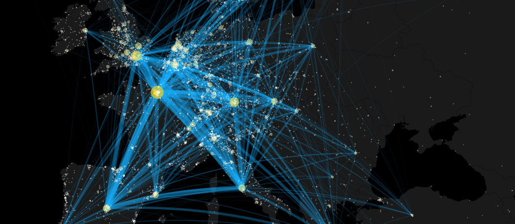
The plan is to do the following

Put Europe on the map
Place a dot at every location that received some funds. Scale the size of the point proportional to the sqrt of the total funds
Draw a line between the cities that have been collaborating in the same project. Scale the width of the line proportional to the number of times those two cities have collaborated

Draw a map of Europe (roughly)

map("world", col="#232323", fill=TRUE, bg="#000000", 
    lwd=0.05, xlim = c(-15, +45), ylim = c(35, 71))

Add the points

To add the data I’m going to create two functions that aid mapping data to aesthetic values. It’s a natural part of ggplot but since I’m using map I have to implement it myself, I think.

The function scl is for scaling intervals to intervals. Argument i1 is the first interval, i2 is the second interval, trans is a transformation function, and ... is all additional parameters that will go to trans. It returns a function that scales values to the desired scale.

scl <- function(i1, i2 = c(0.05, 10), trans = I, ...){
  function(x) trans((x - i1[1]) / diff(i1), ...) * diff(i2) + i2[1]
}

The second function make_color_scale() makes use of scl() and scales numeric intervals to specific colors and alpha values, this makes it easy to generate gradients.

make_color_scale <- function(colors = c("black", "skyblue"), 
                             alphas = c("ff", "ff"), 
                             n_colors = 256,
                             trans = I, ...){
  # Function that returns a color scale function
  # Usage example:
  #  test_scale = make_color_scale()
  #  n = 1000
  #  plot(x = 1:n, y = 1:n, col = test_scale(1:n), pch=20)
  
  color_pal <- colorRampPalette(colors)(n_colors)
  alphas_hex <- str_c("#", alphas, alphas, alphas, sep = "")
  alpha_pal <- str_extract(colorRampPalette(alphas_hex)(n_colors), ".{2}$")
  total_pal <- str_c(color_pal, alpha_pal)
  
  function(x, rng = range(x)) total_pal[round(scl(rng, c(1, n_colors), trans, ...)(x))]
}

Ok, now for drawing some points

#draw the map
map("world", col="#232323", fill=TRUE, bg="#000000", 
    lwd=0.05, xlim = c(-15, +45), ylim = c(35, 71), asp=1)

#Create color scale
point_color_scale <- make_color_scale(colors = c("white", "gold"), 
                                      alpha = c("55", "aa"), 
                                      trans = sqrt)

#Create point size scaler
cex_scale <- scl(range(city_contributions$city_contribution), 
                 c(0.1, 3), 
                 trans=sqrt)

#Draw the points
city_contributions %$%
  points(lon, lat, pch=20, 
         col = point_color_scale(city_contribution), 
         cex = cex_scale(city_contribution))

Add collaboration network

Let’s draw an arc on the map between two cities if there exists a project where institutions from those two cities are collaborating.

First, find all of the projects that have no collaborators in any other city

singles <- organizations %>% 
  group_by(rcn) %>%
  summarise(n = n_distinct(address)) %>%
  filter(n == 1)

nrow(singles)

## [1] 13762

Remove the singles using because they won’t have any connections. anti_join removes all rows from the first dataset that don’t have a match in the second

collaborators <- organizations %>%
  anti_join(singles, by = "rcn")

Next we have to expand the data frame to include all pairs of cities within each project. Let’s break this task apart and first define a function that does this for one single data_frame

make_network <- function(df) {
  #This function takes data_frame as an input
  #and has to return another data frame that includes all
  #unique pairs of locations (rows) together with coordinates
  
  #Some projects have institutions from just a single city,
  #Return NULL in this case
  df_unique <- df %>%
    count(lon, lat)
  
  if(nrow(df_unique) == 1) return(NULL)
  
  #Compute all unordered pairs between the rows
  df %>% 
    unite(lonlat, lon, lat, sep="|") %>% 
    count(lonlat) %$% 
    combn(lonlat, 2) %>% 
    t() %>% 
    as_data_frame %>%
    separate(V1, into=c("lon1", "lat1"), sep = "\\|", convert = T) %>%
    separate(V2, into=c("lon2", "lat2"), sep = "\\|", convert = T)
}

Now let’s split the collaborators dataset by rcn, apply make_network on each split, and combine the results back to one data_frame. This might take a couple of seconds.

collaboration_network <- collaborators %>%
  split(.$rcn) %>%
  map_df(~ make_network(.x))

Drawing all those lines one by one would take forever. Let’s instead encode the number of projects between the same cities into line width

collaboration_network <- collaboration_network %>%
  count(lon1, lat1, lon2, lat2)

Let’s throw out connections that have less than 50 projects and at least one endpoint is outside the drawn area, i.e. Europe

cnx <- collaboration_network %>%
  filter(n >= 50) %>%
  filter( between(lon1, -15, 45) &
          between(lat1, 35, 71) |
          between(lon2, -15, 45) &
          between(lat2, 35, 71)) %>% 
  arrange(n)

We have 1025 edges left with the count ranging between 50 and 836. Time to draw them. For drawing the great circle arcs I’m using gcIntermediate function from geosphere package. I’m also defining new scaling function for line colors and line width

map("world", col="#232323", fill=TRUE, bg="#000000", 
    lwd=0.05, xlim = c(-15, +45), ylim = c(35, 71))

#Connection line color scaler
cnx_color_scale = make_color_scale(c("deepskyblue"), 
                                   c("11", "88"), 
                                   trans = sqrt)

#line width scaler
rng = range(cnx$n)
lwd_scale = scl(rng, c(0.3, 10))

for(i in 1:nrow(cnx)){
  # Interpolate the great circle lines
  inter2 <- gcIntermediate(c(cnx$lon1[i],
                             cnx$lat1[i]),
                           c(cnx$lon2[i],
                             cnx$lat2[i]), n=30,
                           addStartEnd=TRUE)
  
  lines(inter2, col=cnx_color_scale(cnx$n[i], rng), 
        lwd=lwd_scale(cnx$n[i]))
}

#Point color scaler
point_color_scale <- make_color_scale(colors = c("white", "gold"), 
                                      alpha = c("55", "aa"), 
                                      trans = sqrt)

#Point size scaler
cex_scale <- scl(range(city_contributions$city_contribution), 
                 c(0.2, 3), 
                 trans=sqrt)

city_contributions %$%
  points(lon, lat, pch=20, 
         col=point_color_scale(city_contribution), 
         cex=cex_scale(city_contribution))

And there we have it.

Discussion

At some point I will try to generate the same image by using ggplot and ggmap etc in order to stay true to the gg way of the world.

The problem so far has been that drawing this partial map of Europe. The country borders are polygons and if Russia for example in its vastness is not entirely in the limits of the plot the whole polygon will be dropped. I would have to cut it with a rectangle representing the plot edges.